
What is a JPEG?
JPEG is an abbreviation for the Joint Photographic Experts Group, which published the original specification in 1992 based on earlier research papers and patents from the mid-1980s.
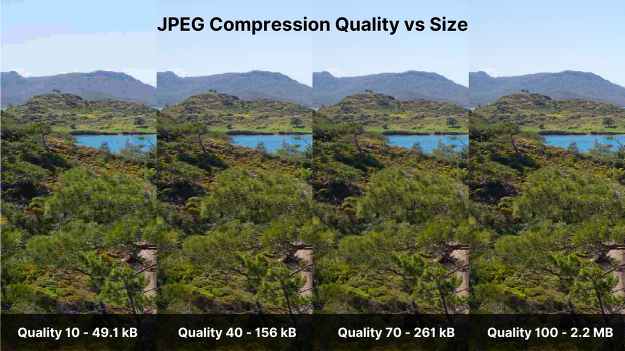
JPEG is a standardized specification for lossy compression for digital images. The compression level can be adjusted, allowing for a trade-off between image quality and file size.
Lossy compression means that JPEG images lose data when saved. This data is lost forever, and the original can never be reformed.
The image below (high resolution) shows a file size reduction of 93% with an image quality of 40 (out of 100).
Impressive, right?
It is for precisely this reason that JPEG is one of the most used “image extensions” on the web.

But it gets better.
Progressive JPEGs combine JPEG compression with interlaced loading.
As a result, progressive JPEGs appear to load faster than their standard JPEG counterparts because they load in progressive waves.
We discuss this in detail in a separate article on Progressive JPEGs.
JPEG is not a File Format
While most people refer to an image being a JPEG file, you might be surprised to know that it is not actually a file format.
JPEG is a compression specification or method, much like the codec you would use in a video.
Most people are, in fact, talking about a JPEG File Interchange Format file or JFIF for short. This is the wrapper that holds the compressed data created by the JPEG compression.

JFIF files are commonly used for web images.
There is also the EXIF format. Photographers commonly use this as it can store information about the photo in its metadata.

Most people do not distinguish between EXIF and JFIF when discussing JPEG files, as both file formats use the .jpeg extension.
Let’s look at both of these formats in turn.
JFIF File Format
The Joint Photographic Experts Group created the JPEG, which is a complex specification of how to compress image data.
The specification has many different options, but its complexity makes it very difficult to implement.
As a result, many " options " were rarely used, such as progressive JPEGs, sequential JPEG files, and different color spaces.

Then in late 1991, a group at C-Cube Microsystems, led by Eric Hamilton, published the JFIF specification. Version 2 was finalized on September 1, 1992, and is still used today.
The Joint Photographic Experts Group and Ecma International took on responsibility for the specification in 2009 to avoid it being lost after C-Cube Microsystems ceased to exist. The latest specification can be found here.
JFIF defines several details left out by the JPEG specification:
- Component sample registration.
- Resolution and aspect ratio.
- Color space.
As such, JFIF became widely adopted as the de facto standard.
We’ll discuss these later in the article when we look at JPEG encoding.
EXIF File Format
The EXIF format is often used by photographers and camera manufacturers to embed various metadata into the image.
The metadata tags are defined in the EXIF specification and include:
- Camera settings: Such as the camera make and model, orientation (rotation), aperture, shutter speed, focal length, metering mode, and ISO speed information.
- Image metrics: Pixel dimensions, resolution, colorspace, and file size.
- Date and time: Digital cameras will record the current date and time and save this in the metadata.
- Location information.
- Thumbnail: Used for previewing the picture on the camera’s LCD screen, in file managers, or in photo manipulation software.
- Description.
- Copyright information.
A .jpeg file can be either an EXIF or JFIF format or even include both formats simultaneously. For example, an EXIF photograph with a JFIF thumbnail.
Due to the extra information stored in the image file, EXIF images tend to be slightly larger than their JFIF counterparts.
The image below shows some of the metadata for this example EXIF file.

JPEG vs. JPG
Before we go on, let’s clear up something that often causes confusion.
There is no difference between the JPG and JPEG extension. Both JPG and JPEG are the same, and the extensions can be used interchangeably.
Before Windows 95, file systems such as MS-DOS only allowed extensions containing 3 upper-case characters.
As such, JPEG was shortened to “JPG”.
Macs, UNIX, Amiga, etc., never had this restriction on file name extensions, so all continued to use the JPEG extension.
Even though the original restrictions are no longer present, both extensions are commonly used today.
How does JPEG Encoding Work?
In this section, I will look at a high level, the broad steps that go into JPEG compression.
As I have discussed previously, many of the options available in the JPEG Standard specification are not commonly used due to their complexity. As such, most image software uses the more simple JFIF format.
This article’s references to JPEG compression or encoding refer to the JFIF format.
JPEG compression encoding can be broken down into several processes, as shown below:

Let’s look at each of the processes in more detail.
JPEG Encoding: Color Transformation
The first stage of JPEG compression is the colorspace transformation.
A colorspace represents a specific organization of colors that can be represented by a color model.
A color model is a mathematical formula used to calculate those colors and can be represented in different ways.
For example, in the image below, the same color is represented by two different color models: RGB format (3 numbers) and CMYK format (4 digits).

These two color models work differently:
- RGB creates white when all the colors are added together (additive), and is used by screens, such as TVs and computer monitors.
- CMYK creates black when all the colors are added together (subtractive) and is used by the print industry.

The most important thing to take away from this is that you can easily convert one color model to another.
JPEG encoding uses this fact to convert from the RGB color model to the YCbCr color model.
Why the YCbCr Color Model?
The human eye is much more sensitive to fine variations in brightness (luminance) than to changes in color (chroma).

JPEG can take advantage of this by converting to the YCbCr color model, which splits the luminance from the chroma. We can then apply stronger compression to the chroma channels with less effect on image quality.
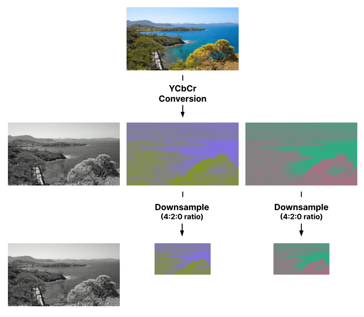
The YCbCr color model converts from the RGB color model and consists of 3 separate categories:
- Luminance (Y) - The luminance data from each red, green, and blue RGB channel is extracted and separated from the chroma data and combined to make the Luminance (Y) channel. The Y channel, by itself, contains enough data to create a complete black-and-white image.
- Chroma Blue (Cb) - The Chroma Blue Channel is the RGB blue channel minus the luminance.
- Chroma Red (Cr) - The Chroma Red Channel is the RGB blue channel minus the luminance.
After subtracting the Y, Cb, and Cb channels from the image, the remainder provides the chroma green information. This can be mathematically extracted instead of encoded, saving bandwidth.
Let’s see how this looks in practice.

As you can see, most of the information in the image is contained in the Y channel.
The next step is to downsample the Chroma Cb and Cr channels.
JPEG Encoding: Chroma Subsampling
This section will look at the process of chroma subsampling and what it looks like in practice.
You can even use our JPEG subsampling tool to try it yourself.
Let’s get started.
Chroma subsampling, or downsampling, is where the color information in an image’s Cb and Cr channels is sampled at a lower resolution than the original.
There are several commonly used subsampling ratios for JPEGs, including:
- 4:4:4 - no subsampling
- 4:2:2 - reduction by half in the horizontal direction (50% area reduction)
- 4:2:0 - reduction by half in both the horizontal and vertical directions (75% area reduction)
- 4:1:1 - reduction by a quarter in the horizontal direction (75% area reduction)
As you can see, the subsampling ratio is expressed in three parts (J:a:b), where:
- J - is the horizontal sampling reference, which is usually four pixels.
- a - is the number of chrominance samples (Cr, Cb) in the first row of J pixels.
- b - is the change between the first and second row of chrominance pixels. This must either be zero or equal a.
You can visualize how this works in the following diagram:

Contrasting colors and luminance in the diagram are used for illustration purposes.
Let’s see how subsampling looks in practice:
The level of subsampling, or whether it is used at all, may depend on the software and settings used to create the JPEG file.
For instance, some graphics software may choose not to use subsampling at higher quality levels.
Where subsampling is carried out, the process is lossy. In other words, pixels are lost and can never be recovered.
Chroma Subsampling Image Size Reduction
Chroma subsampling can provide sizable file size savings for very little difference to how the image looks.
As you can see from the images below (original high resolution), the human eye can see no noticeable difference between the two.
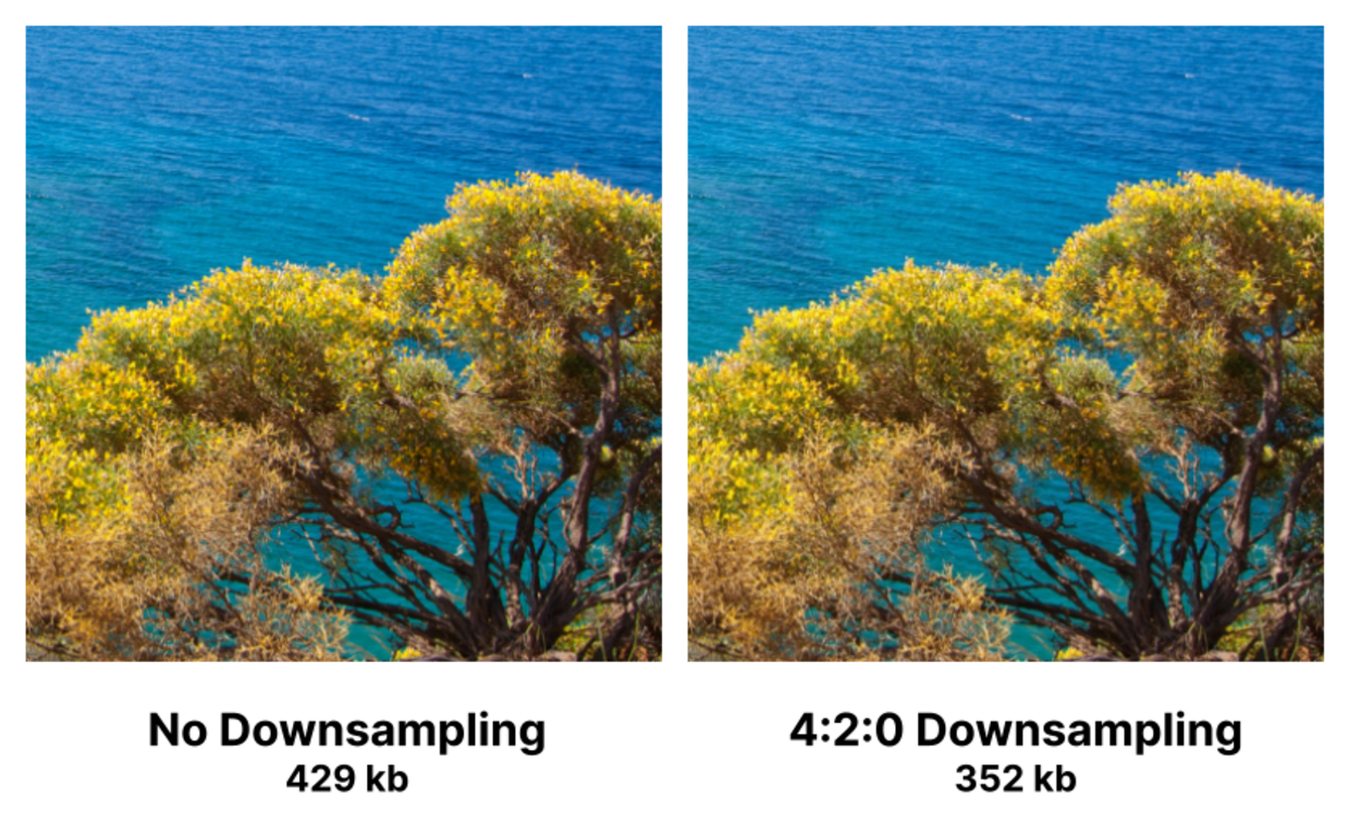
Let’s compare the file size between the original and the downsampled images (remember, this is before the rest of the JPEG encoding process). We get a file size saving of 17.9%.
Perhaps a more realistic comparison would be to compare the file sizes of the two images after the entire JPEG encoding process is complete.
For this, I will use the Cloudinary image service to convert the original image to two JPEGs at the max quality (100), one with subsampling and one without subsampling.
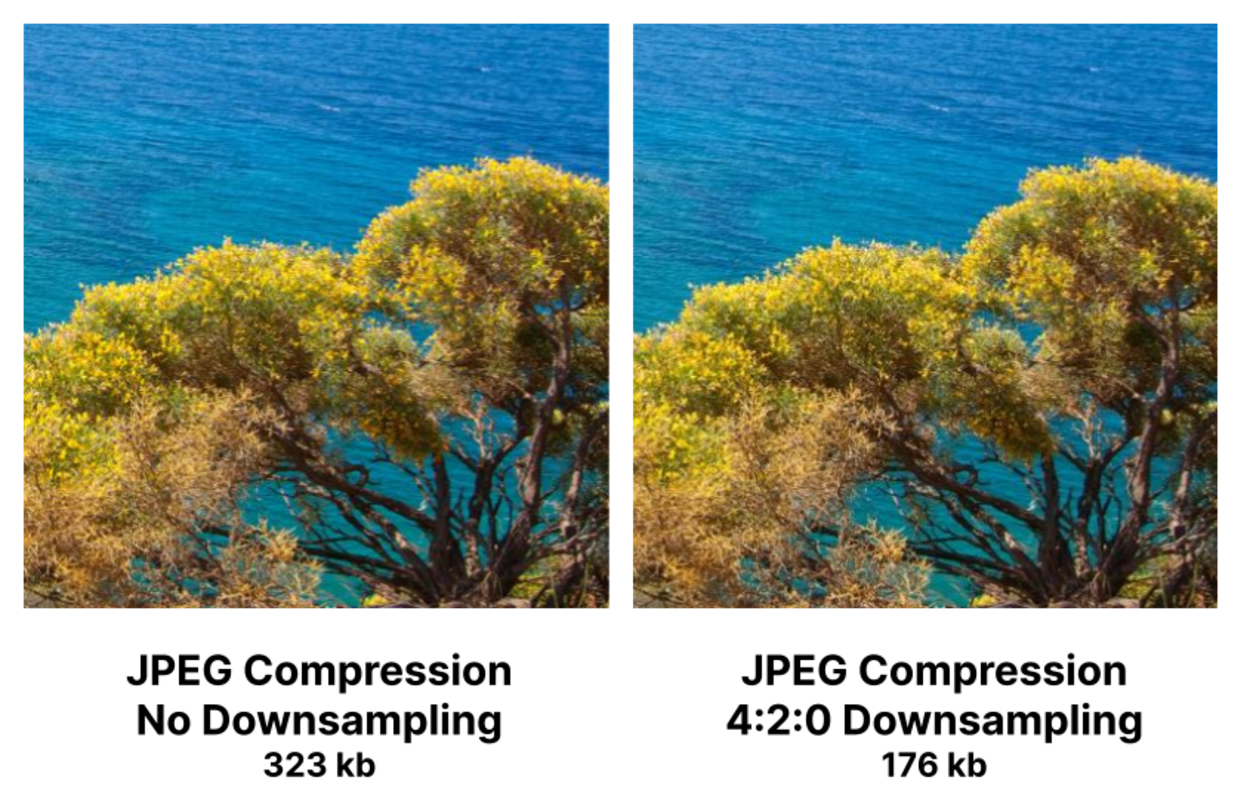
As you can see, the file size difference between the non-downsampled JPEG image and downsampled JPEG image is significantly better, with a saving of 45.5%.
Pretty impressive, right?
As I previously mentioned, Chroma Subsampling is lossy, which means that some data is lost forever in the process.
In the following video, you can see two images; one with no subsampling and the other with 4:2:0 subsampling.
As the video zooms in, you can see some degradation in the subsampled image beginning to appear.
It is noticeable where the colors in the image abruptly change, but only at significant magnification.
Chroma subsampling would be beneficial for this type of image.
Try this example for yourself with our Chroma Subsampling tool.
However, color degradation and other artifacts can be very noticeable in some situations.
This may be why, in 2015, when Akamai’s Colin Bendell ran a test on 1 million JPEGs he discovered that nearly 60% of the images did not use subsampling at all. Furthermore, only around 39% of the images used 4:2:0.
Let’s look at the chroma subsampling artifacts in more detail.
Chroma Subsampling Artifacts
Having reduced the image resolution, the next step is to enlarge the chroma channels back to their original size.
Not only have you lost pixel data during the subsampling process, but the pixel data will be changed again when the image is resized back to the original dimensions.
The process of enlarging the image by creating new pixels is called resampling.
At this stage, the first artifacts start to appear, including aliasing (jagged edges), blurring, and edge halos.

These artifacts are most visible where there is a bold transition between colors.
How does resampling work?
In simple terms, resampling (from a 4:2:0 ratio) takes the original pixel and replaces it with four average-weighted color pixels.
In essence, colors are mixed and may become much less vibrant.
The following diagram shows, in simplistic terms, how this looks.

Various resampling methods can help reduce the impact of these artifacts, including nearest neighbor, bicubic, bilinear, Lanczos, and more.
Your software will usually decide which method to use during this subsampling process.
When to avoid Chroma Subsampling
Chroma subsampling can suffer from artifacts in certain situations, such as image text or other places where colors change abruptly.
Abrupt Color Change Artifacts
Chroma subsampling should be avoided when the image contains colors that change abruptly. This may include logos, diagrams, or items with sharp edges on contrasting backgrounds.
This can be seen in the example below between the green and magenta border. The first image is unsampled.

The second image shows the first image subsampled at 4:2:0 and edited to show a zoomed cross-section.

Try this example with our chroma subsampling tool.
Image Text Artifacts
Chroma subsampling should be avoided when using colored text or text on colored backgrounds.
Let’s look at this affect using a popular test pattern from Rtings (high resolution):
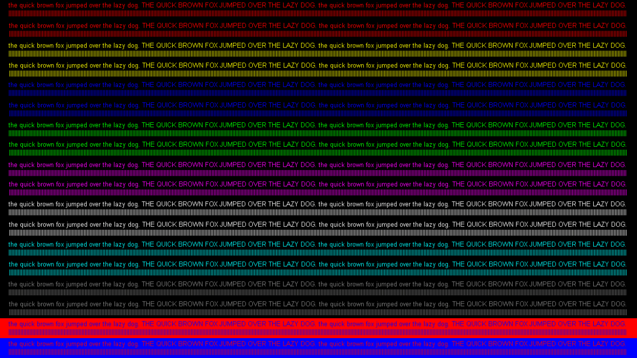
All the text in this image is fully readable, and the colors are vibrant.
Now let’s look at the image after it has been subsampled at 4:2:0 (high resolution):
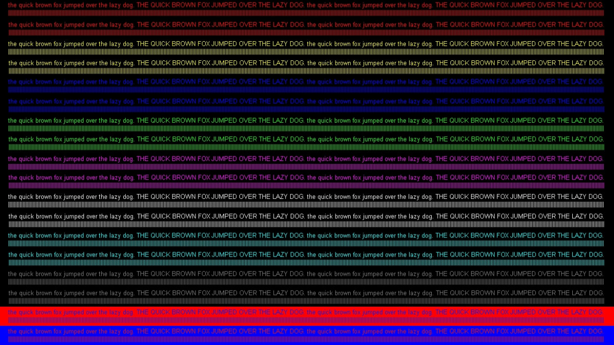
You will notice that much of the text colors now look dull.
Try this example with our chroma subsampling tool.
Summary
In summary, you may wish to avoid chroma subsampling in the following situations:
- Where the image contains many areas where colors change abruptly. For example, diagrams, logos, and race cars containing styling or advertising.
- Where the image contains color text or text on a colored background. For example, tutorial screenshots and logos.
Throughout the rest of the JPEG encoding process, the Y, Cb, and Cr color channels are processed separately.
Try it for yourself
Use the tool below (or our full-screen version) to show \ hide the Y, Cb, and Cr channels, as well as change the subsampling ratio.
Try changing the chroma ratio, or vary the resampling filters.
JPEG Encoding: Block Splitting
Block splitting is the process of splitting each channel in a source image into pixel blocks called Minimum Coded Units (MCU).
Each channel may have a different-sized MCU, depending on whether that channel was subsampled.
For example, here is the MCU size for the following subsampling ratios:
- 4:4:4 - 8 x 8 pixels
- 4:2:2 - 16 * 8 pixels
- 4:2:0 - 16 * 16 pixels
Increasing the MCU size when an image is subsampled makes sense. For example, with 4:2:0 chroma subsampling, each block of 4 pixels is averaged into a single color.
Let’s look at an 8 x 8 pixel MCU for the luminance channel.
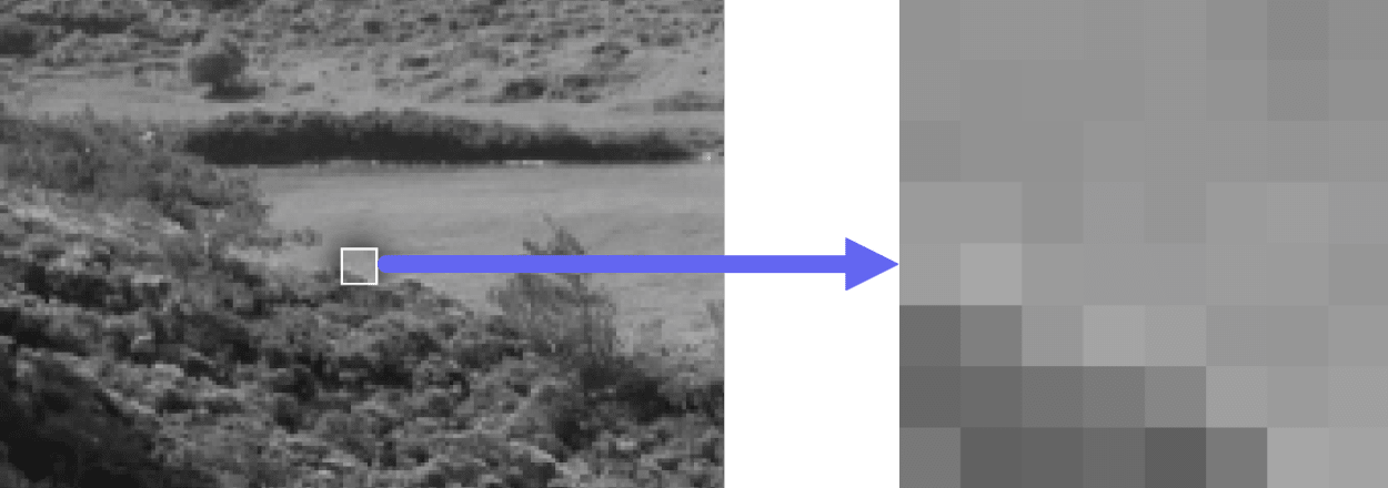
The image on the left shows the MCU in the context of the zoomed-in part of the image. The right-hand image shows the zoomed-in portion.
What if the image does not divide exactly into MCU blocks?
For JPEG compression algorithms to work, images must only contain complete MCU blocks.
In other words, the image dimensions must be multiples of an MCU, for example, 8 pixels for the 4:4:4 subsampling ratio. For example, an image with a size of 501 x 375 pixels must first be changed to an image with a size of 504 x 376 pixels.
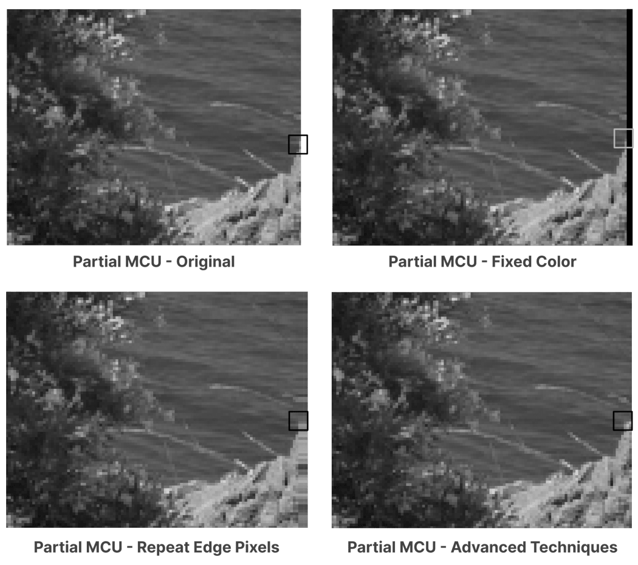
If the image has partial MCU blocks, then the software encoding the JPEG image must add its own dummy data to those blocks.
The data (or padding) added to the image depends on the software, but the following techniques may be used:
- Use a fixed color, such as black.
- Repeat the pixels at the edge of the image (the most common technique).
- More sophisticated techniques.
These techniques can be seen in the following image:
Once the dummy data is added, the blocks go through the rest of the JPEG encoding process.
Finally, the additional pixels are removed.
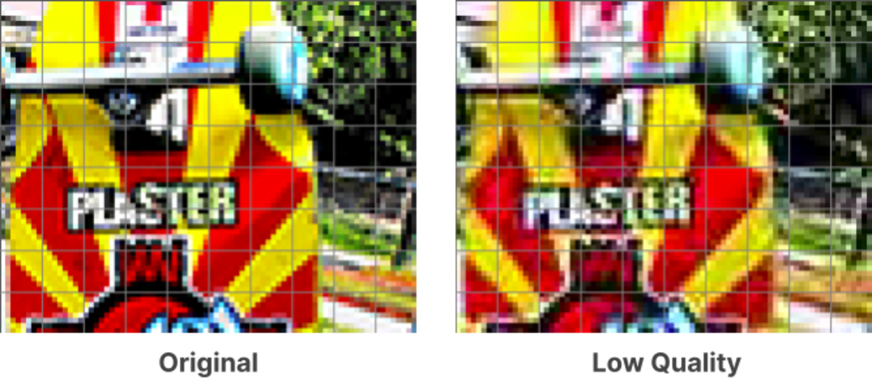
Blocking artifacts
In certain circumstances, the division of the image into MCUs may cause some visual discontinuities.
For example, the edges of the MCUs may be visible if the JPEG has been compressed at very low quality.
This can be seen in the following image:

Let’s overlay the boundaries to make it clearer:
As you can see, along the boundaries of the MCUs, you can see some abrupt changes in color and \ or intensity.
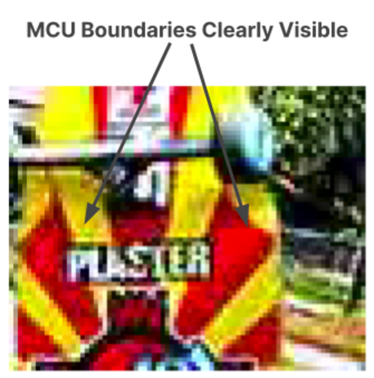
This arises because each MCU is compressed separately, with differing amounts of information discarded from each.
Fortunately, though, this is only an issue when using the lowest-quality settings.
JPEG Encoding: Discrete Cosine Transform (DCT)
This is where the real magic starts to happen.
Each 8x8 pixel block of each channel (Y, Cb, Cr) is converted from a spatial domain representation to a frequency domain representation using a two-dimensional type-II discrete cosine transform (otherwise known as “type-II DCT”).
This won’t make much sense right now, so let’s look at it in more detail, starting with some basic concepts.
What is a Cosine Function?
A cosine function, such as y=cos(x), goes between 1 and -1 on the Y axis, and 0 to 𝝅, then 2𝝅, and so on.
This cosine function can be visualized in the following diagram as a wave:

As you can see, when x=0, y=1. At x=𝝅, y=-1. Finally, at x=2𝝅, y=1 again. This pattern then repeats.
What is a Discrete Cosine Transform?
The way that discrete cosine transform works is that we take image data and we try to represent it as the sum of multiple cosine waves.
It sounds complicated, but I will explain how it all works right now.
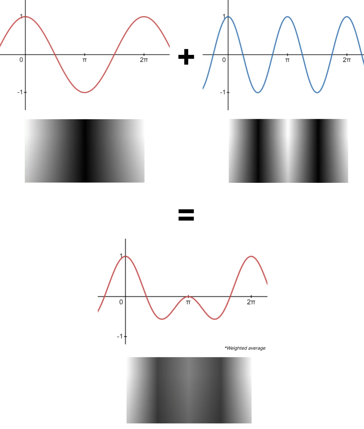
Let’s imagine we have the standard cosine wave and a second wave at a much higher frequency.

We get a completely different and much more complex wave if we add them together.

The wave is now twice as tall as the original input, so a weighted average is taken.
In this case, we divided everything by two because we used 2 cosine waves.

And here is what the respective cosine waves would look like in image form.
The above is only the most basic example.
In reality, you can mix more than 2 or more cosine waves together to create much more complex images.
In fact, any 8x8 pixel block can be represented as the sum of a set of weighted (positive or negative) cosine transforms.
As it happens, JPEG uses a set of 64 different cosine values to produce any 8x8 pixel block.
These are visualized below:

Watch the following video to see how 64 different cosine values can be used to represent an 8x8 pixel block.
Let’s take a deeper, more technical look into how this works.
STEP 1. Convert to a Frequency-domain Representation
To carry out calculations on the image, we must first convert each Y, Cb, and Cr channel to a frequency-domain representation.
Here is how it looks:

Each number in the matrix represents a pixel in the 8x8 image. The darker pixels are represented by a lower number, and the lighter pixels have a higher number.
Each number falls between 0 and 255, with the midpoint being 128.
STEP 2. Recenter Around Zero
Before computing the DCT of each 8x8 block, each value in the matrix must be recentered around zero. I.e., the midpoint must be 0.
Each number must, therefore, have 128 subtracted so that the range is between -128 and 127.
Here is how it looks:

The reason for recentering around 0 is to reduce the dynamic range requirements in the DCT calculation stage, which we look at next.
STEP 3. Calculate the Discrete Cosine Transform Coefficients
The next step is to calculate the two-dimensional DCT coefficients, which can be calculated using the following formula:

I’m not going to go into mathematics and what each value in the formula means. But if you want to know more, you can read the wikipedia article here.
Let’s perform this calculation on the example matrix above to get the DCT coefficients.

There are two types of DCT coefficients:
- DC coefficient - This is the top left-hand corner DCT coefficient, otherwise known as the constant component. This defines the basic hue for the entire 8x8 pixel block.
- AC coefficients - These are the remaining 63 DCT coefficients, otherwise known as the alternating components.
The DCT calculation tends to aggregate a larger signal in one corner of the matrix, meaning these cosine waves contribute a larger amount of data to the image.
This is important as it is accentuated in the quantization step.
I’ll touch more on this in the next section.
Summary
Before we proceed to the final two steps, it is helpful to recap what we have learned.
Here is what we know:
- JPEG compression uses a standard set of 64 cosine functions.
- The 8x8 image (or sub-image) is converted to a frequency-domain representation in the form of an 8x8 matrix.
- The frequency-domain representation is recentered around 0 by deducting 128 from each figure.
- The DCT Coefficients are then calculated.
At this point, any 8x8 image can be created by adding together a weighted set of 64 cosine functions. The cosine functions are weighted by their respective DCT coefficients that were just calculated.
However, there are two more steps in the compression process before the JPEG image is created.
Let’s look at these now.
JPEG Encoding: Quantization
The quantization process aims to reduce the overall size of the DCT coefficients so that they can be more efficiently compressed in the final Entropy Coding stage.
Quantization relies on the principle that humans are better at seeing small differences in brightness over a larger area but not so good at distinguishing high-frequency brightness variations.
You can see the high-frequency cosine functions at the bottom right of the following image:
Now let’s compare these high-frequency cosine functions with the DCT coefficients we previously calculated:
You can see that the coefficients in the bottom right of the frequency domain matrix have a much smaller influence on the final image than the low-frequency coefficients in the top left.
The quantization process uses this fact to significantly reduce the amount of information in the high-frequency components. It does this by dividing the DCT coefficient by the quantization matrix.
Quantization Matrix
The quantization matrix determines the compression ratio, otherwise known as the quality setting (usually 0-100).
To calculate the quantized DCT coefficients, you divide the DCT coefficients by the quantization matrix. The result is then rounded to the nearest whole number.
Each of the Y (luminance), Cb (chroma blue), and Cr (chroma red) channels are calculated separately.
There are two quantization tables in a JPEG image. One for the luminance channel and one for the chrominance channels.
A typical Luminance channel quantization matrix for a quality of 50% (as specified in the JPEG standard) looks as follows:

For the Chrominance channels, the following quantization matrix is used:

The higher the values in the matrix, the greater compression and the lower the quality.
The quantization matrices used when encoding a JPEG are stored in the image. This is because the same ones are required for the decoding process, which I discuss later in this section.
The next step is to use these matrices to quantize the DCT coefficients.
Let’s do this now.
Quantize the DCT Coefficients
To calculate the quantized DCT coefficients, you must divide the DCT coefficients by the quantization table and then round to the nearest whole number.
Here is the calculation:
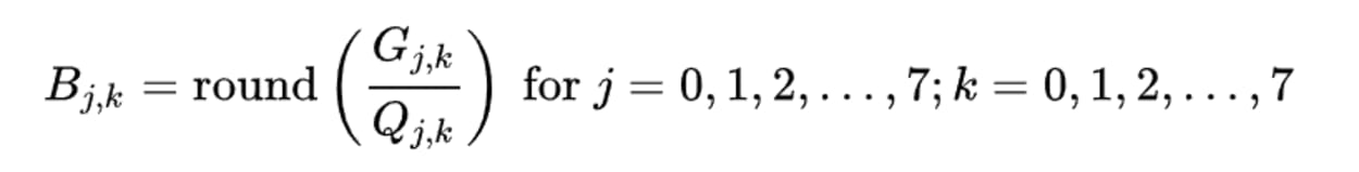
Where:
- B = The quantized DCT coefficients
- G = The DCT coefficients
- B = The quantization matrix
Let’s do an example calculation for the top left item in the Luminance DCT coefficients matrix (-415.37) at 50% quality.
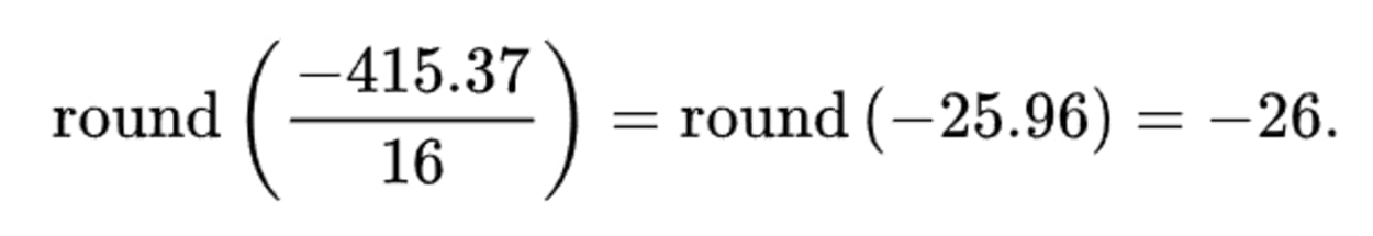
Which, when used on the entire DCT coefficient matrix, gives the following:

As you can see, only 20 cosine functions now affect the image. Many high-frequency components have been rounded to zero, with the others reduced to single digits.
Because of this, the number of bits (1’s and 0’s) required to store the image is significantly reduced, reducing the JPEG file size.
Other than chroma subsampling, this quantization step is the only loss of data (lossy operation) in the entire JPEG compression process.
The amount of data loss in the image depends on the quantization table used or, more simply, the quality level.
The Quantization Effect on Image Quality
Here is how image compression affects the quality of an image:
| Image | Quality | Size | Compression Ratio |
|---|---|---|---|
 | Highest quality (100) | 81.4 kb | 2.7:1 |
 | High quality (50) | 14.7 kb | 15:1 |
 | Medium quality (25) | 9.4 kb | 23:1 |
 | Low quality (10) | 4.8 kb | 46:1 |
 | Lowest quality (100) | 1.5 kb | 144:1 |
You will need to make some kind of personal judgment as to what level of quality is most suitable for your image.
Try it for yourself
The quantization process and the impact of the quality setting can be seen in our quantization tool below.
To use select an image, then click on any part of the image to load the 8x8 pixel block. The 64 cosine functions used to build the image are shown underneath.
Try adjusting the quality lower to see how some of the cosine functions no longer contribute to the image and how that affects the look of the image.
You can also adjust the “phase” slider to see how the image builds up over time.
Summary
Before we proceed to the final step, let’s review what we have learned:
- The purpose of quantization is to reduce the size of the DCT coefficients.
- The quantization Matrix determines the compression ratio or quality setting. Each quality setting has its own matrix.
- Two quantization Matrices are required to encode a JPEG image. One for the Luminance channel. The other is for the Chroma channels.
- Both these matrices are stored in the encoded image. They are required during the decoding process.
- To calculate the quantized DCT coefficients, you must divide the DCT coefficients by the quantization table and then round to the nearest whole number.
- Many high-frequency components in the quantized DCT matrix get rounded to zero, with the others reduced to single digits. This significantly reduces the size of the image.
The final stage takes the quantized DCT matrix and applies lossless entropy coding to further reduce the size of the image file.
Let’s look at this now.
JPEG Encoding: Entropy Coding
Entropy coding is a form of lossless data compression.
It consists of two parts:
- Arranging the quantized DCT coefficients in a zigzag order
- Employing run-length and applying Huffman coding.
JPEG uses a method of coding that combines the run-length and amplitude information into a single Huffman code.
Let’s look at how this works.
Arrange the Quantized DCT Coefficients in a Zigzag Order
The order in which the coefficients are processed during run-length coding matters.
Let’s look at our previous example.
If we order the coefficients horizontally, we get the following:

- -26 -3 -6 2 2 -1 0 0 0 0 0 1 1 -4 -2 0 -3 1 5 -1 -1 0 0 0 0 0 0 0 -1 2 1 -3 1 0 0 0 0 0 0 0 0 0 0 0 0 0 0 0 0 0 0 0 0 0 0 0 0 0 0 0 0 0 0 0
If we order the coefficients in a zigzag pattern, we get the following:

- −26 −3 0 −3 −2 −6 2 −4 1 −3 1 1 5 1 2 −1 1 −1 2 0 0 0 0 0 −1 −1 0 0 0 0 0 0 0 0 0 0 0 0 0 0 0 0 0 0 0 0 0 0 0 0 0 0 0 0 0 0 0 0 0 0 0 0 0 0
Notice how there is a longer string of zeros next to each other in the latter method.
It turns out that the zigzag pattern is better at grouping similar frequencies together.
Next, we need to carry out run-length encoding and Huffman coding.
Apply Run-length encoding and Huffman Coding on AC Coefficients
Run-length encoding is a form of lossless compression in which data sequences are stored as a single data value and count rather than in their original form.
The run-length works by removing zeros from the data sequence and recording how many zeros came before the next item in the series.
Run-length coding utilizes the following format:
- (RUNLENGTH, SIZE)(AMPLITUDE);
Where:
- x is the non-zero quantized AC coefficient
- RUNLENGTH is the number of zeros that come before x.
- SIZE is the number of bits required to represent x. I.e., no. of characters.
- AMPLITUDE is the bit-representation of x
This will make more sense if we look at the previous examples.
Take the following text:
- −26 −3 0 −3 −2 −6 2 −4 1 −3 1 1 5 1 2 −1 1 −1 2 0 0 0 0 0 −1 −1 0 0 0 0 0 0 0 0 0 0 0 0 0 0 0 0 0 0 0 0 0 0 0 0 0 0 0 0 0 0 0 0 0 0 0 0 0 0
When we apply run-length encoding with a zigzag order, we get the following:
- (0, 2)(-3);(1, 2)(-3);(0, 1)(-2);(0, 2)(-6);(0, 1)(2);(0, 1)(-4);(0, 1)(1);(0, 2)(-3);(0, 1)(1);(0, 1)(1);(0, 2)(5);(0, 1)(1);(0, 1)(2);(0, 1)(-1);(0, 1)(1);(0, 1)(-1);(0, 1)(2);(5, 1)(-1);(0, 1)(-1);(0, 0);
Note the following:
The first number is the DC coefficient. This is dealt with differently, and I’ll come on to this momentarily.
If you follow the amplitudes for the above it goes “-3, -3,-2 …”, instead of “-3, 0, -3, -2”. Note how the first zero is omitted from the sequence.
This is because it is represented by RUNLENGTH in the second item in the sequence “(1, 2)(-3). The run length, in this case, is 1, denoting a zero comes before the amplitude of “-3”.
Huffman code words
You may have wondered where the last entry, “(0, 0);” comes from in the previous example.
- (0, 2)(-3);(1, 2)(-3);(0, 1)(-2);(0, 2)(-6);(0, 1)(2);(0, 1)(-4);(0, 1)(1);(0, 2)(-3);(0, 1)(1);(0, 1)(1);(0, 2)(5);(0, 1)(1);(0, 1)(2);(0, 1)(-1);(0, 1)(1);(0, 1)(-1);(0, 1)(2);(5, 1)(-1);(0, 1)(-1);(0, 0);
Huffman contains two special code words:
- (0,0); - One is to mark the sequence as ending early where the remaining coefficients are zero. This is otherwise known as “End-of-block” or “EOB”.
- (15, 0)(0) - The other is when the number of zeros exceeds 15 before reaching another non-zero AC coefficient.
Apply Differential Pulse Code Modulation on DC Coefficients
The DC coefficient (the first item in the quantized DCT Coefficient matrix) is omitted when applying Entropy encoding.
This is because it is dealt with in a different manner, called Differential Pulse Code Modulation, or DPCM.
Instead of storing the full value of the DC coefficient for each 8x8 pixel block, the difference between the current and previous block is stored.
Because the variation between DC coefficients is usually not that large, it tends to result in a smaller number being stored, which uses less space.
DPCM is demonstrated in the image below:

Summary
We now have an idea of all the different steps that go into encoding a JPEG image. The following subsection will look at this in reverse and go through the decoding process.
First, though, let’s summarize what we know about Entropy Coding:
- The Quantized DCT Coefficients are processed in a zigzag order.
- The AC coefficients have run-length encoding, and Huffman coding is applied. This works by removing zeros from the data sequence and recording how many zeros came before the next item in the sequence. Huffman applies special code words to further optimize.
- The DC coefficient is encoded differently. Instead of storing the full value of the DC coefficient for each 8x8 pixel block, the difference between the current and previous block is stored.
JPEG Decoding
All the steps must be carried out in reverse order to decode the image.
Let’s go through the process for our previous example.
1. Start with Quantized DCT Coefficient Matrix
After reversing the Entropy Coding stage (including reversing the DC Coefficient differential), we start with the following matrix:
2. Multiply by the Quantization Matrix
There are two Quantization Matrices. One for Luminance and one for Chroma. This example will look at the Luminance channel.
We must use the same quantization matrix that the image was encoded with. In this case, the matrix specified in the JPEG standard for 50% quality. This is shown below.
The resulting matrix is as follows:

3. Calculate the Two-dimensional Inverse DCT (2D type-III DCT)
In the encoding step, we calculated the Discrete Cosine Transform (DCT) using a type-II DCT.
In this step, we calculate the inverse of this previous calculation, otherwise known as a type-III DCT. We do this with the following formula, and again you can read more about the mathematics behind this calculation on Wikipedia.
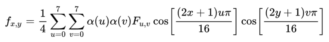
If we apply this formula to our matrix, we get the following:

Add 128 to each entry in the matrix
During encoding, we recentered the coefficients in the matrix around zero by deducting 128 from each figure.
This final step reverses this by adding 128 to each entry.

If the decompression process is lower than zero or greater than 255, the figures are clipped to that range.
Comparing the original with the decompressed image
Even at 50% quality settings, the image between the original and JPEG compressed image is still relatively similar.

Let’s see how this image compares:

As you can see, there are some differences, especially in the top left and bottom left of the image.
However, bearing in mind this image is really just 8x8 pixels, the difference between the two images is minimal.
JPEG images work well with all modern browsers, including Chrome, Firefox, Safari, and Edge.
The only browser with significant issues with the progressive format is Internet Explorer, version 8, and below.
Those Internet Explorer versions will still display progressive images only after downloading the entire image file.
JPEG Browser Support
All known web browsers widely support JPEG image files.
Other JPEG formats, such as JPEG XR, JPEG XL, and JPEG 2000, are not currently supported by most web browsers at this time.
Desktop Browser Support
| Chrome | Edge | Firefox | IE | Opera | Safari |
|---|---|---|---|---|---|
| Yes | Yes | Yes | Yes* | Yes | Yes |
* From version 9.
Mobile Browser Support
| Android Webview | Chrome Android | Edge | Firefox Mobile | IE Mobile | Opera Mobile | Safari Mobile |
|---|---|---|---|---|---|---|
| Yes | Yes | Yes | Yes | Yes | Yes | Yes |